This tutorial examines the concept of the average as a single value representing a collection of values. It focusses on the mean, median, and mode.
The average (especially in physics) can also mean the center or balance point, but, for most everyday use, we tend to think of the average as representative value.
Average comes from the Old French avarie which came from the Old Italian avaria which came from the Arabic awariyah meaning damaged goods or merchandise. Which is probably apt, given how how badly averages are often misused.
The Old French avarie used to mean the damage sustained to a ship or its cargo. The meaning later shifted to mean an equal distribution of the costs of such damage. For example, if ten men pooled money together and hired a ship to bring spices from India and the ship or its goods was damaged, the avarie was the equal distribution of the costs or losses. (In English, we have the expression, “What’s the damage?” when inquiring about the cost of something. Although this comes from the Latin damnum meaning loss or fine, the intent is quite similar to the original meaning of avarie.
An average is a single value that is representative of a collection of values. For an average to be meaningful, it shouldn’t have any surprises.
For example, if you have a box of apples, and want to know how much an individual apple weighs: you weigh the apples (8Kg), divide by the number of apples (40) and arrive at a value of 200g per apple.
You reasonably expect that each apple you pull out will weigh about 200g – some might be a little heavier, some might be a little lighter. You do not expect to pull out apples that weigh 25g or 500g. If you did, you would probably believe you had been deceived.
NOTE: I won’t discuss it here, but you can give additional information, like the standard deviation and confidence interval to more precisely qualify the average. But then this becomes more of a discussion on statistics.
Mean
When people think about averages, the mean (also called arithmetic average or arithmetic mean) is what comes to mind.
Mean comes from the Latin medianus which means middle. If the data is well distributed, then the mean will be in the middle of the values.
You add up all the values and divide by the total number of values.
In math speak it might look like this:
[latex]\mathbf{\frac{\sum_{1}^{n} X}{n}} [/latex]
While mathematical equations might look intimidating, they’re not really. The Σ symbol just means sum (add) up all the following values. The X stands for all the values to be added. The little 1 and n on the Σ symbol tell us to do the summation from the first value to the nth value. Finally, the n in the denominator tells you to divide the sum by n (the total number of values).
For example, given the following ages of children in a grade 5 class (it’s small class), what is the average age?
10, 11, 11, 11, 11, 10, 11, 11, 11, 10, 11, 11, 11, 11, 11
The total sum is 162.
Divided by the number of students (15), the answer is 10.8.
The answer isn’t too surprising, since most children are around 11 years old in grade 5.
Suppose that as well as having the age of the children we also have the age of the teacher (an older one, nearing retirement):
Given the following ages in a grade 5 class, what is the average age?
10, 11, 11, 11, 11, 10, 11, 11, 11, 10, 11, 11, 11, 11, 11, 60
The total sum is 222.
Divided by the number of ages (16), the answer is 13.875.
This average is rather surprising because the age is almost 3 years older than you would expect for a grade 5 class. This happens because the average was skewed (distorted) by an outlier.
An outlier is a value that is significantly outside the range of all the other values. Sometimes outliers significantly affect the result, sometimes they do not.
If the number of students in the class had been 40 (a very large class), the outlier would have had less of an effect (adding a little over year to the average age). If the age had been lower (say a young teacher aged 24), the average age would have been 11.625 – maybe a little high, but not too surprising.
Another case where outliers may affect a result is the average salary at a small store. Suppose the owner earns $150,000 per year and the 5 clerks each earn between $18,000 and $24,000 per year, if you include the owners salary in the average, the result is higher than it really should be.
One way to deal with this is to ignore any outliers and calculate the average age as we did before. If we do this, then we must be clear that one or more values were excluded and explain why they were excluded from the calculation.
The mean is the preferred average since it uses all the values, but it can be sensitive to outliers.
Median
The median is another way of determining the average and works well if we have outlying values.
Median comes from the Latin medianus meaning middle. It comes from exactly the same root as mean, but, in this case, the median is exactly in the middle of the values.
To calculate the median, you sort the values in order from smallest to largest and then pick the middle value.
Given the following ages in a grade 5 class, what is the median age?
10, 11, 11, 11, 11, 10, 11, 11, 11, 10, 11, 11, 11, 11, 11
Sorted in order the ages are:
10, 10, 10, 11, 11, 11, 11, 11, 11, 11, 11, 11, 11, 11, 11
As we see, the middle value is 11.
The answer isn’t too surprising, since most children are around 11 years old in grade 5.
The median value differs from the mean value above. This will usually be the case, although the difference should be quite small.
Given the following ages in a grade 5 class, what is the average age?
10, 11, 11, 11, 11, 10, 11, 11, 11, 10, 11, 11, 11, 11, 11, 60
Sorted in order the ages are:
10, 10, 10, 11, 11, 11, 11, 11, 11, 11, 11, 11, 11, 11, 11, 60
Because we have an even number of values, there is no value exactly in the middle. In this case, we take the two middle values and calculate their mean:
11 + 11 = 22
22 / 2 = 11
Unlike the mean calculation above, this average was not sensitive to the outlier value and we get the (unsurprising) value of 11 years.
The median works well when the data is fairly uniform, doesn’t have too many outliers, and doesn’t have large gaps in the middle.
Mode
The mode is the most different of the averages – it is the one we tend to instinctively give as an answer.
Mode comes from the Middle English moede which comes from the Latin modus meaning manner or measure.
If you are asked what is the average age of students in a grade 5 class, you would most likely answer 11 years old (not 10.8 as we saw in the first example).
If you are asked how many children the average woman has, you would most likely answer 1 or 2 or 3 (depending on what your experience is). The only time you would answer 1.7 or 2.3 (or whatever number statistics show us) is if you have been taught that number.
For example, how many desserts does the average person order in a restaurant? You will probably answer “one”. Not 0.78 (or some such number) – even though you know that not all people order a dessert and a few people might order more than one.
The mode is the most popular number.
The mode is determined by ordering all the numbers and then counting the number of times each number occurs. The number that occurs the most times is the mode.
Given the following ages in a grade 5 class, what is the average age?
10, 11, 11, 11, 11, 10, 11, 11, 11, 10, 11, 11, 11, 11, 11, 60
Sorted in order the ages are:
10, 10, 10, 11, 11, 11, 11, 11, 11, 11, 11, 11, 11, 11, 11, 60
The ages occurs with the following frequency:
The age 10 occurs 3 times.
The age 11 occurs 12 times.
The age 60 occurs 1 time.
The mode of this data set is 11.
In this data set, the mode is the same as the median, but it doesn’t have to be.
If no number is more popular than another (they all have the same count / frequency, or two or more have the same count / frequency), then there is no mode.
In some cases, multi-modal distributions are considered. The most common is bimodal where there are two modes (equally popular numbers).
Given the ages of children in a Summer camp, what is the average (mode) age?
9, 10, 9, 10, 12, 10, 11, 12, 10, 9, 12, 12, 11
Sorted in order the ages are:
9, 9, 9, 10, 10, 10, 10, 11, 11, 12, 12, 12, 12
The ages occur with the following frequency:
The age 9 occurs 3 times.
The age 10 occurs 4 times.
The age 11 occurs 2 times.
The age 12 occurs 4 times.
In this case, there is no mode, since the ages 10 and 12 occur with equal frequency.
As mentioned earlier, sometimes multi-modal distributions are considered valid. In this case, this is a bimodal distribution with the ages 10 and 12 being the most popular.
Sometimes the mode will return the wrong value or answer.
Consider the following counts of dessert choices at a restaurant:
No dessert: 8:
Apple Pie: 7:
Icecream: 5:
Brownie: 6:
If asked to pick the most popular dessert, by using the mode, you would answer that no dessert was the most popular option – even though 18 people chose some sort of dessert and only 8 didn’t choose a dessert.
Why be Careful With Averages?
It is always important to make sure that when we give an average that the average is meaningful.
Consider the following ages of grandparents and grandchildren at a play group (one child per grandparent):
1, 1, 1, 2, 2, 2, 3, 3, 3, 3, 3, 50, 52, 55, 55, 57, 58, 59, 59, 60, 61, 65
What is the average age?
Mean: 655 / 22 = 29.77
Median: (50 + 3) / 2 = 26.5
Mode: 3
Which “average” age most accurately reflects the age at the play group?
It definitely is not the mean or median. The mode reflects most accurately the age of the intended users of the play group, but it does miss grandparents.
A better way to present this “average” would be to split the data into two groups and report each one independently.
Summary
Mean
Pros: uses all the data. Finds the “true” center of all the data.
Cons: sensitive to outliers in the data
Median
Pros: finds the middle value. Reasonably insensitive to outliers.
Cons: does not consider all the data. Doesn’t work well if there are large gaps in the middle.
Mode
Pros: finds the most popular value.
Cons: no answer if there is no single most popular value. Sensitive to frequency (count) of values. Does not consider all the data.
Are the Mean, Median and Mode ever the Same Value?
In theory, if your data is normally distributed (Guassian / bell curve) then the mean, median, and mode will all be identical.
In practice, we rarely get perfect data, so they will differ slightly.
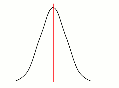
In the image above, the mean, median, and mode are identical – the red line in the middle.
NOTE: The mode only exists if the data above is discrete rather than continuous.
Are Half the Values Greater and Half the Values Smaller than the Average?
In theory, yes, in practice this is only true if (1) the values follow a normal distribution, or (2) the median is taken.